Getting started

This is a very short guide on how to get started with Karamelo.

How to install Karamelo?

In order to use Karamelo, you need to download, extract and compile Karamelo's source code. Compiling is no that complicated thanks to the use of CMake (cmake.org). It will automatically check for most dependencies, but unfortunately not all of them.

Dependencies

Karamelo has a few dependencies that need to be satisfied for it to successfully compile and run. They are:

• Cmake
• MPI. It was tested with OpenMPI
• Eigen version 3
• Boost which can be easily installed with the package manager of every Linux distribution.
• Python 3 with Matplotlib
• matplotlib-cpp which allows the use of the Matplotlib library directly from C++.
  Remark: a bug was detected that prevent versions of matplotlib-cpp earlier than f4ad842e to be used with Karamelo.
• gzstream which is used to compress dump files.

Installing Karamelo on Ubuntu

The authors, as many researchers that do simulation work use Linux, and Ubuntu in particular. In order to make it simple for people like us to install and run Karamelo on Ubuntu, here are the steps to follow to download, build, and run the last version of the code. The following steps were tested using the versions 18.04 LTS and 16.04 LTS.

1. Install all the dependencies shipped with ubuntu:

   sudo apt install make gcc g++ libz-dev cmake libopenmpi-dev libeigen3-dev libboost-dev python-dev python-matplotlib

2. Download and install the extra external dependencies:
   1. Matplotlib-cpp:

      git clone https://github.com/lava/matplotlib-cpp.git 

      Matplotlib-cpp being just a collection of headers, there is nothing to compile. However, one needs to celect the right commit that allows karamelo to run without problems. More recent commits have been found to be buggy:

      cd matplotlib-cpp/
      git checkout f4ad842e

   2. Download gzstream and compile it.

3. Add the path to Eigen, gzstream and matplotlib to your paths: Add to your .bash_profile:

   CPATH=$CPATH:/usr/include/eigen3:/home/toto/gzstream:/home/toto/matplotlib-cpp:/usr/include/python2.7
   export CPATH
   
   LIBRARY_PATH=$LIBRARY_PATH:/usr/include/eigen3:/home/toto/gzstream:/home/toto/matplotlib-cpp:/usr/include/python2.7
   export LIBRARY_PATH

   Remark: change /home/toto/ to the path to the root directory where you have installed gzstream and matplotlib-cpp (they can be different from each other).

4. Download and install Karamelo:

   git clone https://github.com/adevaucorbeil/karamelo.git
   cd ~/karamelo
   cmake -DCMAKE_BUILD_TYPE=release build .
   make

5. Enjoy!

A simple first example

Here is a simple example of two disks bouncing onto each other to get you started with Karamelo.

Setup

This example involves two elastic disks launched at a speed 0.1 mm/s towards each other:

Input file

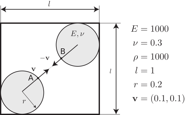
In order to simulate this problem, we need to create an input file that we called two-disks.mpm which reads:

#####################################################
#               UNITS: MPa, mm, s                   #
#####################################################
E   = 1e+3
nu  = 0.3
rho = 1000
K      = E/(3*(1-2*nu))
mu     = E/(2*(1+nu))
lambda = E*nu/((1+nu)*(1-2*nu))
c      = sqrt(E/rho)
L    = 1
hL   = 0.5*L
A_zy = L*L
FLIP=1.0
#---------- SET METHOD --------------#
method(ulmpm, FLIP, linear, FLIP)
N        = 20     # 20 cells per direction
cellsize = L/N    # cell size
# 2D problem, which the computational domain is
dimension(2,-hL, hL, -hL, hL, cellsize)
# solids (2 balls)
R = 0.2
region(rBall1, cylinder, -hL+R, -hL+R, R)
region(rBall2, cylinder, hL-R, hL-R, R)
material(mat1, linear, rho, E, nu)

#---------- SET SOLID --------------#
ppc1d = 2
solid(sBall1, region, rBall1, ppc1d, mat1, cellsize,0)
solid(sBall2, region, rBall2, ppc1d, mat1, cellsize,0)

#---------- IMPOSE INITIAL CONDITIONS --------------#
group(gBall1, particles, region, rBall1, solid, sBall1)
group(gBall2, particles, region, rBall2, solid, sBall2)
v = 0.1
fix(v0Ball1, initial_velocity_particles, gBall1, v, v, NULL)
fix(v0Ball2, initial_velocity_particles, gBall2, -v, -v, NULL)

#-----------OUTPUT-------------------------------------#
N_log = 50
dumping_interval = N_log*1
dump(dump1, all, particle, dumping_interval, dump_p.*.LAMMPS, x, y, z)
dump(dump2, all, grid, dumping_interval, dump_g.*.LAMMPS, x, y, z)

fix(Ek, kinetic_energy, all)
fix(Es, strain_energy, all)
Etot = Ek_s + Es_s

#----------- RUN --------------------#
set_dt(0.001)

log_modify(custom, step, dt, time, Ek_s, Es_s)
plot(Ek, N_log, time, Ek_s)
plot(Es, N_log, time, Es_s)
plot(Etot, N_log, time, Etot)
save_plot(plot.pdf)

set_output(N_log)

run_time(3.5)

Running

In order to run this example, on 4 CPUs, for instance, simply execute the following command:

NUM_CPU = 4
mpirun -np ${NUM_CPU} /path/to/karamelo/directory/karamelo -i two-disks.mpm

Of course, you can change the number of CPU by adjusting the variable NUM_CPU.

Results

This example generates three types of results:

1. A log file called log.mpm
   The data displayed in this file are specified by the command:

   log_modify(custom, step, dt, time, Ek_s, Es_s)

   Therefore, here they are, in order: the step (step), the timestep (dt), the overall time (time), the total kinetic energy (Ek_s) and the total strain energy (Es_s)
2. Two series of dump files called dump_p.*.LAMMPS and dump_g.*.LAMMPS to be visualized with Ovito. The first series contains particles data, the second, grid nodes data. They are generated by the following commands:
   

   dump(dump1, all, particle, dumping_interval, dump_p.*.LAMMPS, x, y, z)
   dump(dump2, all, grid, dumping_interval, dump_g.*.LAMMPS, x, y, z)

3. A plot of the kinetic, strain, and total energies, saved as "plot.pdf". This is obtained with the following commands:
   

   plot(Ek, N_log, time, Ek_s)
   plot(Es, N_log, time, Es_s)
   plot(Etot, N_log, time, Etot)
   save_plot(plot.pdf)